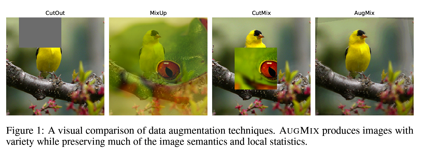
TL;DR
In machine learning, we use a set of data (known as the “training” data) to teach an algorithm how to solve a task. In this context, we’re talking about deep neural networks which are a kind of machine learning algorithm designed to classify images. An image classifier’s job is to look at an image and decide which category it belongs to, like identifying whether a photo is of a cat or a dog.
When the algorithm is learning, it adjusts itself to perform well on the training data. It’s then tested on separate “test” data to see how well it has learned. Ideally, the training and test data should be very similar (identically distributed) in nature. For example, if the task is to distinguish between cats and dogs, and if all the images in the training set are taken in broad daylight, we expect the test set also to have images taken in similar conditions.
However, in real-world scenarios, there can be a mismatch between the training and test data. This could be due to a variety of factors like the lighting conditions, the angle of the camera, or the breed of the dogs and cats in the images. When this mismatch happens, the accuracy of the image classifier can drop significantly because it has not encountered these conditions during training.
Most current techniques for training these algorithms struggle when the test data is different from the training data in ways they didn’t anticipate. This is where the technique called “AUGMIX” comes in.
AUGMIX is a method that helps improve the robustness of the model. Robustness in this context refers to the model’s ability to maintain accuracy even when the test data differs from the training data in unexpected ways.
Here’s how AUGMIX works: it applies a mix of augmentations (slight modifications) to the images in the training data. These might include things like adjusting the brightness or contrast, rotating the image, or zooming in slightly. By doing this, AUGMIX creates a wide range of scenarios the model might encounter. It’s like showing the model not only pictures of cats and dogs taken in the day but also at twilight, from different angles, of different breeds, etc.
This helps in two ways:
- It makes the model more robust because it has seen a wider range of image conditions during training.
- It helps the model to provide better uncertainty estimates. Uncertainty estimates tell us how confident the model is about its predictions. A well-calibrated model knows when it’s likely to be wrong, which is very useful when decisions based on these predictions have significant consequences.
The Problem
-
Machine Learning Models and Training Data: Machine learning models are like students. They learn from a book (training data) and they’re expected to use that knowledge to solve problems (make predictions) in the real world (deployment). It’s very important that the book is representative of the real world, otherwise, they’ll struggle to solve real-world problems correctly.
-
Mismatch between Training and Test Data: Imagine if a student studied from a book about mammals but was then tested on birds. The student would likely fail because the test (test data) doesn’t match what they learned (training data). The same thing can happen with machine learning models. But even though this problem is common, it’s not studied enough. As a result, machine learning models often struggle when they encounter data that’s different from what they were trained on.
-
Data Corruption: Just a little bit of change or “corruption” to the data (like a bird wearing a hat in the test data when the book only had birds without hats) can confuse the machine learning model (classifier). There aren’t a lot of techniques available yet to make these models more resistant to such changes.
-
Uncertainty Quantification: Some machine learning models (like probabilistic and Bayesian neural networks) try to also measure how sure they are about their predictions (uncertainty). But these models can also struggle when the data shifts because they weren’t trained on similar examples.
-
Corruption-Specific Training: Training a model with a focus on specific corruptions (like birds wearing specific types of hats) encourages the model to only remember these specific corruptions and not learn a general ability to handle any kind of hat.
-
Data Augmentation: Some people propose aggressively changing the training data (aggressive data augmentation) to prepare the model for all kinds of changes it might encounter. But this approach can require a lot of computational resources.
-
Trade-off between Accuracy, Robustness, and Uncertainty: Chun et al. (2019) found that many techniques that improve the model’s test score (clean accuracy) make it less able to handle data corruption (robustness). Similarly, techniques that make a model more robust often make it worse at estimating how sure it is about its predictions (uncertainty). So there’s often a trade-off between accuracy, robustness, and uncertainty.
The Solution
-
AUGMIX: This is a new technique that manages to hit a sweet spot. It improves the model’s ability to handle data corruption (robustness) and its ability to estimate how sure it is about its predictions (uncertainty), all while maintaining or even improving its test score (accuracy). And it does this on standard benchmark datasets, which are datasets commonly used to test machine learning models.
-
How AUGMIX Works: AUGMIX uses randomness (stochasticity) and a wide variety of changes (diverse augmentations) to the training data. It also uses a special type of loss function called Jensen-Shannon Divergence consistency loss, which is a mathematical way to measure how different two probability distributions are. Furthermore, it mixes multiple changed versions of an image to achieve great performance. It’s like showing the model different versions of the same image (like a cat in different lighting conditions, from different angles, etc.) and teaching it that they are all still the same category (a cat).
-
AUGMIX Results on ImageNet: ImageNet is a popular benchmark dataset for image classifiers. AUGMIX achieves the best performance so far on this dataset in terms of handling data corruption. It also reduces perturbation instability from 57.2% to 37.4%. Perturbation instability is a measure of how much small changes to the input (like slightly changing the color of an image) affect the model’s predictions. A high perturbation instability means the model’s predictions change a lot even for small changes to the input, which is not desirable. By reducing this from 57.2% to 37.4%, AUGMIX makes the model more stable and reliable.
-
Offocial code released at : https://github.com/google-research/augmix
AUGMIX
What’s the hype?
Let’s try to understand why, what and how
-
AUGMIX: This is a technique used to change the training data (data augmentation) to make the model stronger (improve robustness) and better at estimating how sure it is about its predictions (uncertainty estimates). The great thing about AUGMIX is that it can be easily added to existing training procedures (training pipelines).
-
Components of AUGMIX: AUGMIX is characterized by two main components. The first is the use of simple changes (augmentation operations) to the images in the training data. The second is a special mathematical measure called a consistency loss, which I’ll explain later.
-
Stochastic Sampling: AUGMIX doesn’t just apply one change to an image, but layers many different changes to the same image. Which changes it applies is decided randomly (sampled stochastically). This produces a wide variety of changed versions of the same image.
-
Consistent Embedding: When the model looks at an image, it converts it into a numerical representation called an embedding. AUGMIX enforces that the model produces a similar embedding for all the changed versions of the same image. This makes sense because, regardless of the changes, it’s still the same image.
-
Jensen-Shannon Divergence: This is the special mathematical measure (consistency loss) used by AUGMIX. It measures how different two probability distributions are. In this case, it’s used to measure how different the model’s predictions are for the different changed versions of the same image. The goal is to make this divergence as small as possible, which means the model is consistent in its predictions for the changed versions of the same image.
-
Mixing Augmentations: This refers to applying several changes (augmentations) to the same image at once. This can produce a wide range of different versions of the same image. This diversity is crucial for making the model stronger (inducing robustness). This is because a common issue with deep learning models is that they tend to memorize the specific changes they see during training (fixed augmentations), instead of learning to handle changes in general.
-
Previous Methods: Earlier techniques tried to increase this diversity by applying a series of different changes one after the other (composing augmentation primitives in a chain). But this can quickly distort the image too much (cause the image to degrade and drift off the data manifold), making it harder for the model to learn from it. You can see an illustration of this in Figure 3 (not provided here).
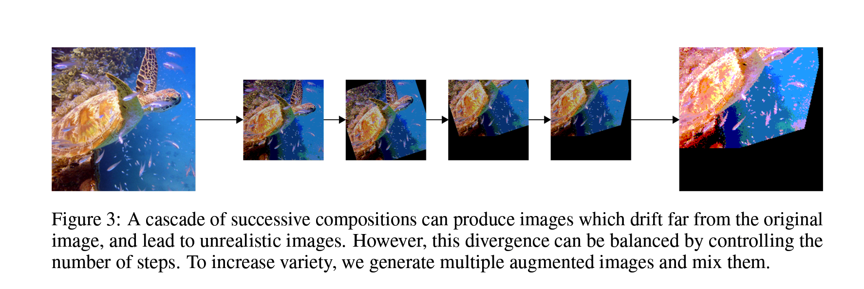
- Mitigating Image Degradation: AUGMIX has a clever solution to this issue. It maintains the diversity of changes without distorting the image too much by mixing the results of several chains of changes (augmentation chains) together. It does this by creating a blend (convex combination) of several differently changed versions of the same image. This keeps the diversity of changes high, but ensures the changed images still resemble the original image, making it easier for the model to learn from them.
Algorithm
1. Input: Model ^p, Classification Loss L, Image xorig, Operations O={rotate,...,posterize}
2. Function AugmentAndMix(xorig, k=3, α=1):
    * Fill xaug with zeros.
    * Sample mixing weights (w1, w2, ..., wk) ~ Dirichlet(α, α, ..., α).
    * For i = 1, ..., k do:
        * Sample operations op1, op2, op3 ~ O.
        * Compose operations with varying depth op12 = op2◦op1 and op123 = op3◦op2◦op1.
        * Sample uniformly from one of these operations chain ∼ {op1, op12, op123}.
        * xaug += wi·chain(xorig) Addition is elementwise.
    * End for.
    * Sample weight m ~ Beta(α, α).
    * Interpolate with rule xaugmix = mxorig + (1 - m)xaug.
    * Return xaugmix.
    * End function.
3. xaugmix1 = AugmentAndMix(xorig) xaugmix1 is stochastically generated.
4. xaugmix2 = AugmentAndMix(xorig) xaugmix1 = xaugmix2.
5. Loss Output: L(ˆp(y|xorig), y) + λJensen-Shannon(ˆp(y|xorig); ˆp(y|xaugmix1); ˆp(y|xaugmix2))
What this means?
- The input to the algorithm is a model ^p, a classification loss L, an image xorig, and a set of operations O.
- The function AugmentAndMix takes an image xorig and generates a new image xaugmix that is a mix of several augmented versions of xorig.
- The algorithm generates two augmented images xaugmix1 and xaugmix2.
- The loss function is a combination of the classification loss L and a Jensen-Shannon divergence between the predictions of the model on the original image xorig and the two augmented images xaugmix1 and xaugmix2.
As stated before the algorithm is thus a data augmentation technique that can be used to improve the robustness and uncertainty estimates of machine learning models. It works by generating a diverse set of augmented images from a single input image, and then training the model on these augmented images. This helps the model to learn to generalize to unseen data, and to produce more accurate uncertainty estimates.
The entire steps are visualised below:
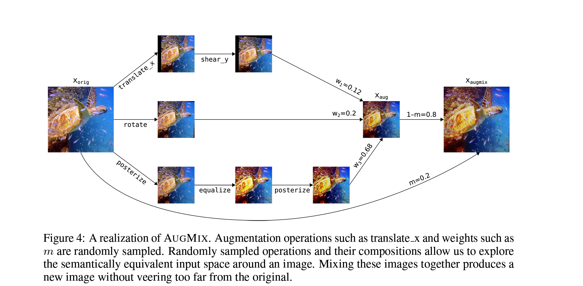
NOTE: The Semantically equivalent space around an image is the image equivalent of a word being surrounded by its synonyms, in meme language think of this as the function saying copy my homework but change it a bit. 
Drilling Down
There are three major steps involved in AUGMIX. These are:
- Augmentations
- Mixing
- Jensen-Shannon Divergence Consistency Loss 💀
Here is what these steps entail in details:
Augmentations
This is the process of changing or altering the images in your training dataset. In the case of AUGMIX, this involves mixing together the results of several different chains of changes (augmentation chains) applied to the same image.
-
AutoAugment Operations: AUGMIX uses a specific set of changes (operations) from something called AutoAugment, which is another data augmentation method. These operations include different ways to change an image.
-
Exclusions: Some of these operations are removed because they overlap with certain types of changes (corruptions) in the ImageNet-C dataset (a test dataset). In particular, changes that affect the image’s contrast, color, brightness, sharpness, and cutout operations are removed. This is done so that the model doesn’t see these changes until it’s being tested. Additionally, operations that add noise to the image or blur it are also not used.
-
Rotate Operation: Some operations can be applied with varying degrees of severity. For example, the rotate operation can rotate the image by a small amount (like 2 degrees) or a larger amount (like -15 degrees).
-
Sampling Severities: For operations that have varying degrees of severity, the severity is chosen randomly each time the operation is applied.
-
Sampling Augmentation Chains: Next, a number of augmentation chains are selected randomly. By default, this number (k) is 3. An augmentation chain is a sequence of one to three randomly selected operations applied to the image.
To put it in simpler terms, imagine you’re an artist with a picture, and you want to create slightly different versions of it. You have a set of tools (operations) you can use to change the picture (like rotating it, zooming in, etc.), but some tools (like changing the color or blurring it) are off-limits. Each time you work on a picture, you can use up to three tools in a sequence (an augmentation chain), and you create three versions of the picture by default. Some tools can be used gently or aggressively (varying severities), and each time you use them, you randomly decide how gentle or aggressive to be.

Mixing
After the images have been changed using the augmentation chains, they’re combined together. This is the mixing step. While there were other options, the method they chose was elementwise convex combinations. It’s a bit like mixing paint colors: you’re blending different versions of an image together.
-
Convex Coefficients: The way you blend the images is determined by a set of weights (convex coefficients). This is a fancy way of saying how much of each image you take when you’re blending them. These weights are chosen randomly from a type of probability distribution called a Dirichlet distribution.
-
Skip Connection: After the images have been mixed, they are combined with the original image using a skip connection. This basically means that the original image is included in the final mixed image. The way the mixed image and the original image are combined is also determined by a weight, which is randomly chosen from another type of probability distribution called a Beta distribution.
-
Multiple Sources of Randomness: There are several factors that are randomly decided in this process: which changes to apply to the image (choice of operations), how severe these changes are (severity of operations), how many changes to apply in a sequence (length of augmentation chains), and how the changed images are blended together (mixing weights).
To simplify, think about making a smoothie. You choose a few different fruits (operations), decide how much of each to use (severity), mix a few different smoothie recipes together (augmentation chains), and then decide how much of each recipe to use in the final smoothie (mixing weights). Then, you add some of the original fruits back in (skip connection) as toppings, this helps to make sure some parts of the original taste is retained 😉.

Jensen-Shannon Divergence Consistency Loss 💀
-
Loss and Smoother Responses: We know that “loss” is like a penalty for the model. The higher the loss, the worse the model is doing. The aim is to get a lower penalty or “loss”. In this case, they want the penalty to enforce “smoother” responses. This means that small changes to an image shouldn’t result in big changes to what the model predicts about the image.
-
Preserving Semantic Content: With AUGMIX, even if we change an image a bit (like turning it or adding noise), the overall subject of the image (like a dog or a cat) stays the same. So, they want the model to predict similar things for the original and the changed images.
-
Minimizing Jensen-Shannon Divergence: This is the penalty they use to make sure the model makes similar predictions for the original and changed images. Here’s the formula:
L(porig,y) + λJS(porig; paugmix1; paugmix2)
Here’s what it means:
-
L(porig, y): This is how different the model’s predictions for the original image (porig) are from what they should be (y).
-
JS(porig; paugmix1; paugmix2): This is how different the model’s predictions for the original and the two changed images are from each other.
-
λ: This is a number that decides how much importance they give to making the predictions similar (JS part) compared to getting the predictions for the original image right (L part).
-
Interpreting the Loss: Imagine you have three people who all look very similar. If you can’t tell which is which based on how they look (porig, paugmix1, paugmix2), then the model is doing a good job. The Jensen-Shannon divergence measures this.
-
Computing the Loss: First, they calculate an “average prediction” (M) from the predictions for the original and changed images. Then, they calculate how different each prediction is from this average.
M=(porig + paugmix1 + paugmix2) / 3 JS(porig; paugmix1; paugmix2)=1/3 (KL[porig||M] + KL[paugmix1||M] + KL[paugmix2||M])
Here, KL (see KL divergence) is another way to measure how different two things are (in this case, the prediction and the average prediction).
-
Upper Bounded Divergence: The Jensen-Shannon divergence can’t be bigger than the log of the number of classes (the number of different things the model can predict, like cat, dog, etc.). This means it’s a good, stable measure to use.
-
Stable, Consistent, and Insensitive Model: This fancy penalty (Jensen-Shannon Consistency Loss) encourages the model to be stable (not change predictions drastically), consistent (predict similar things for similar images), and insensitive (not overreact to small changes in the image).
In simpler terms, imagine the model as a student learning to classify animals in images. The student gets penalized (Jensen-Shannon Consistency Loss) if they drastically change their guess about the animal when they see the same image slightly altered. The aim is to teach the student to be steady and consistent in their learning and not get easily confused by minor changes in the images.
Implementation
Keras CV provides a nice and easy implementation of AugMix that you can try in any of your existing data loading pipelines. Here is a small snippet to get you started:
import keras_cv
import tensorflow_datasets as tfds

# Load the dataset
dataset = tfds.load(
    name="oxford_iiit_pet"
)

# Build the AugMix layer and pass the images through the layer
augmix = keras_cv.layers.preprocessing.AugMix(value_range=(0, 255))
augmix_inputs = augmix(batch_inputs)

keras_cv.visualization.plot_image_gallery(
    images=augmix_inputs["images"],
    value_range=(0, 255),
)
Conclusion
-
AUGMIX: We need to think of AUGMIX like a chef’s special recipe for training a model. The recipe includes creating and mixing together different versions of the same image (like a cake with different toppings), and then teaching the model to recognize these as essentially the same thing. (all chefs are whimsical)
-
State-of-the-art Performance: This technique helps models do really well on some popular tests. These tests are CIFAR-10/100-C, ImageNet-C, CIFAR-10/100-P, and ImageNet-P. Think of them like exams in school, where the model needs to identify objects in images correctly, the different datasets are the different levels in the exams.
-
Calibration: Calibration is like how well the model knows it’s right. A well-calibrated model, when it says “I’m 70% sure this is a cat”, is right about 70% of the time. With AUGMIX, models are really good at this and stay good at it, even when the images they are trying to recognize become a bit different than what they were trained on.
-
Reliable Models: By using AUGMIX, models can be more reliable. This is important especially when models are used in situations where it’s really important they don’t make mistakes, like in self-driving cars or medical diagnoses.
So summing up, AUGMIX is like a special training method (chef’s secret recipe) that helps our models (students) do really well on their exams, keeps them confident about their answers, and makes them reliable even when faced with slightly unfamiliar questions (like an image of a shocked cat). This is especially useful when we need our students to perform tasks where mistakes can lead to serious problems, like AI taking over the world and targeting humans. Just kidding :)
References